


|
STONE: A COMPUTER
PROGRAM FOR THE THREE-DIMENSIONAL SIMULATION OF ROCK-FALLS
by
Federico
Agliardi, Giovanni Corsta, Riccardo Detti & Fausto Guzzetti
Introduction
Rock-falls
pose a continuous hazard in mountain areas world wide. Despite the fact that
rock-falls are a simple landslide type to model, only few attempts have been
made to establish rock-fall hazard and the associated risk at the regional
scale. We developed a 3-dimensional simulation program that starting from
thematic information available in digital format and using GIS technology,
generates simple maps useful to assess rock-fall hazard. The program requires as
input a DTM, the location of rock-fall detachment areas, the dynamic friction
coefficient used to simulate the loss of velocity during rolling, and the
coefficients for normal and tangential energy restitution at the impact points.
The program allows to cope with the natural variability of the input data by
using a random component approach. Outputs of the
program are in raster and vector formats. The former includes the count of
rock-fall trajectories, the maximum velocity and the maximum height computed at
each grid cell. The latter consists of the planar (2-dimensional) and the
3-dimensional trajectories of the rock-falls. The program outputs proved to be
consistent with the results of other rock-fall simulation programs, to be
reliable for modelling rock-falls in 3-dimensional geomorphological settings,
and to effectively aid in the assessment of rock-fall hazard over very large
areas.
The
program STONE
The program STONE
simulates in three-dimensions the fall of a boulder along a slope. The program,
written in ANSI C language, was designed to use thematic data already
available for large areas, or that could be obtained from geological,
geomorphological and land use maps or through reconnaissance investigations, and
to generate spatially distributed information useful to assess rock-fall hazard
at the regional and local scales.
Input data
STONE requires the
following input data:
-
a
DTM, representing topography in raster format;
-
a
raster map (a grid) showing the location of the "starting cells",
i.e., the cells from which rock-falls occur. Values in the grid may range
from 1 to 1000, indicating the number of boulders "launched" from
each starting point (i.e., the number of trajectories computed from each
grid cell). The figure also defines the local frequency of occurrence of
rock-falls. The grid may contain –1 values, indicating cells where a
rock-fall must stop ("stopping cells", e.g., the location of
effective defensive measures, a river in an open flat valley, etc.);
-
two
grids for the normal and tangential restitution coefficients, used to
compute the loss of velocity where the boulder impacts on the ground;
-
a
grid for the dynamic friction coefficient, used to compute the loss of
velocity where the boulder is rolling along the
slope; and
-
a
text file containing initial and controlling parameters .
For convenience, the 5
input grids are provided to the program as ascii (text) files in the Gridascii
format supported by the ArcInfoâ and ArcViewâ GIS softwares.
Cinematic
modelling
STONE
uses a "lumped mass" approach to simulate rock-falls, i.e., the
boulder is considered dimensionless with all the mass concentrated in a point
(the centre of mass). The size, shape and mass of the boulder are not considered
and a cinematic simulation of the rock-fall process is performed. The advantage
of the lumped mass approach lays in its simplicity and in the computational
speed. Taking into account the mass of the boulder, its shape and size would
allow for a complete dynamic modelling, but would introduce uncertainties
(particularly due to the irregular shape of the boulder), would increase the
computation time, and would generate a large variability in the results making
it more difficult to ascertain rock-fall hazard at the regional scale.
The
travel path (or trajectory) of a boulder is computed automatically from the DTM,
without any user involvement. The trajectory depends on the starting point, the
topography, and the coefficients used to simulate the loss of velocity at the
impact point or where the boulder is rolling. To describe topography, the
representation of the terrain based on equally spaced elevation points (DTM) is
subdivided into regular triangles making up a Terrain Regular Network (TRN).
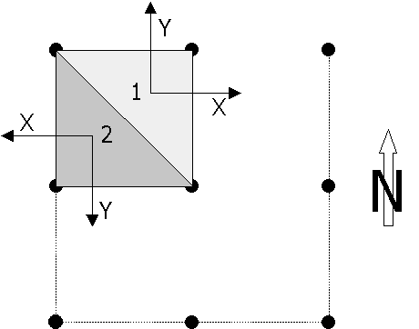
TRN: Triangular Regula
Network. The vector representation of topography used bu STONE.
Triangles
are planar and of two types: type 1 (upper-right triangle) is constructed with
the upper left, upper right and lower right elevation points of each DTM cell;
type 2 (lower-left triangle) is constructed by taking the upper left, lower left
and lower right elevation points. The advantages of using a TRN, i.e., a vector
representation of topography based on regular planar triangles, can be
summarised as follows:
-
A TRN
maximises the information on elevation given by the DTM. Triangles allow for
the detailed tracking of a rock-fall trajectory within a DTM cell, providing
a higher spatial resolution than the original DTM. This is particularly
important if the DTM is coarse.
-
Triangles
allow to use cinematic equations working along slope profiles on a discrete
representation of topography (the DTM).
-
Planar
triangles are easy to compute and are generated only where needed (i.e.,
where a rock-fall trajectory intersects or "flies" over a
triangle), making the computation faster. As a drawback,
triangles may be computed more than once if the trajectories coming from
different source areas cross the same DTM cell.
To compute the rock-fall
trajectory a local cartesian coordinate system is used. The x and y axes of the
local system lay on the local triangle, with the x axis to the right for
triangles of type 1 and to the left for those of type 2, and the y axis pointing
upslope for triangles of type 1 and down slope for those of type 2. The z axis
is perpendicular to the local triangle and points upwards. Appropriate functions
were developed to transform from absolute (latitude, longitude and elevation) to
local (x, y, z) coordinates and back. The use of a local coordinates system
simplifies the calculations and makes the computation faster.
STONE is capable of
modelling three of the four "states" that a rock-fall can take,
namely: free falling, bouncing and rolling. Sliding is not considered because it
represents a (usually) negligible part of a rock-fall. If necessary, sliding
could be modelled by the same equations used to describe rolling, but with
higher friction coefficients.
Starting from a source
cell, STONE "shoots" a boulder horizontally out of the cell along the
steepest slope and at an initial velocity set by the user (usually 0.5 to 2 m
sec-1). High starting velocities can simulate the triggering of
rock-falls by seismic shaking. After the horizontal start, the boulder, driven
by gravity, follows a parabolic (ballistic) trajectory (free falling) until it
hits the ground. Air drag is neglected, for simplicity. The impact
(intersection) point is determined by checking the elevation (z) of the boulder
against the elevation of the local triangle at the same x and y local
coordinates. If a boulder flies over the edge of the local triangle, a nearby
triangle is computed and the trajectory tracked over the new triangle. A
specific algorithm determines which side of the local triangle is crossed and
selects the proper DTM cell to calculate the new triangle.
When the location of the
impact point has been determined, the new direction of the trajectory and the
local velocity components (vx, vy and vz)
of the boulder are computed. The boulder "escape" direction is
obtained by mirroring the incoming direction, i.e., the rebound (or escape)
angle is considered to be equal but opposite to the impact angle. To simulate
the loss of energy at the impact point, the escape velocity components are
computed by multiplying the incoming velocity components by the user-defined
tangential (for x and y components) and normal (for the z component) restitution
coefficients. Normal and tangential components are treated separately for a
better and more flexible simulation of the rock-fall process. Indeed, results of
field experiments show that the normal component is about half of the tangential
component. When the escape direction and velocity have been computed, the
boulder starts a new parabola (i.e., a free fall segment) and a new intersection
point is searched further down slope, inside or outside the local triangle.
STONE simulates rolling
of a bolder on a surface (the local triangle) using a rather simple approach.
The loss of velocity due to the dynamic friction is modelled by a dragging force
acting on the local plain against the direction of movement. The local
coordinates of the boulder and its velocity components along the surface are
computed by iteration, introducing at each time step a dragging (resistance)
force equal to f = sin(atan(Φd))× g, where Φd
is the user-defined dynamic friction angle for the corresponding DTM cell.
STONE determines the
position of a boulder flying or rolling along a slope at successive time
intervals. To track the boulder trajectory accurately the local coordinates (x,
y, z), the velocity and the flying height are computed using an adaptive time
step (D t). The time step (in seconds) is computed as the ratio of the local
velocity (in m·sec-1) and the user defined tabulation steps (in
meters). Tabulation steps are different for free fall and rolling. Thus,
regardless of the velocity, the coordinates and cinematic information along a
rock-fall trajectory are recorded always at the same distance, along the
direction of motion. A peculiar condition arises at the impact point that may
occur during a time step, and not at the end of it. For this reason the last
time step is adjusted to match exactly the impact point.
Since the trajectory of a
rock-fall is a (complex) mixture of free falling, bouncing and rolling, a set of
"conditions" were adopted to switch from one "state" to the
other. Some of the transitions are simple and intuitive, others require an a
priori decision from the user. Transition between free falling and impact is
obvious: it occurs where a boulder impacts (intersects) the topographic surface.
After the impact a boulder is forced to fly (rebound),
unless: the velocity of the boulder is lower than the user defined minimum
velocity, in which case the boulder is stopped; or the velocity of the bolder is
below a user defined threshold (usually set at 5 meters per seconds) and the
span of the last free-fall segment (the parabola) is less than a user defined
value (usually set to 0.1 to 2 meters, depending on the size of the block and
the roughness of the topographic surface). In the latter case the boulder is
considered to be rolling and the appropriate algorithm is used.
Transition between
rolling and free falling is controlled by topography. A boulder that starts
rolling within a local (planar) triangle will keep rolling until
it stops because its velocity falls below the lower velocity threshold,
or it reaches one of the edges of the local triangle. In the latter case the
elevation (z) of the boulder is checked on the next local triangle to see if the
boulder will keep rolling on the new triangle, or if it will fly above it along
a new ballistic trajectory ("jumping" condition). A special case
arises when a boulder rolling out of a local triangle hits a steeper triangle
(steep terrain) in the direction of motion. Where the condition arises,
STONE triggers the "impact"
algorithm whenever the difference between the slope of the incoming trajectory
and the slope of the trajectory on the new triangle is greater than a user
defined value, usually 45 degrees.
Outputs
STONE
outputs the results of its calculations in both raster and vector formats.
Raster outputs are represented by three grids (of the same format and size of
the input grids) showing for each cell: the cumulative count of rock-fall
trajectories that passed through each cell, the highest computed velocity, and
the largest flying height (distance to the ground) computed along the rock-fall
trajectories.
The grid showing the
total number of rock-fall trajectories provides information on the expected
frequency of occurrence of rock-falls. For each grid cell the count of
trajectories is a proxy for the probability of being intercepted
(crossed) by a rock-fall. The larger the number of computed trajectories,
the higher the frequency of occurrence of rock-falls. The grids of the highest
computed velocity and of the largest distance to the ground provide information
on the (maximum) expected intensity of a rock-fall, a proxy for the maximum
kinetic energy expected at each grid cell. Raster outputs are provided in the
same format used for input grids, and are easily read by ArcInfo or ArcView GIS
systems for display, mapping and analysis.
A 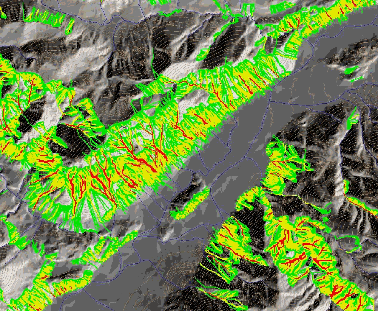
B 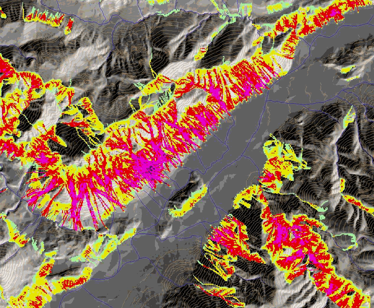
C 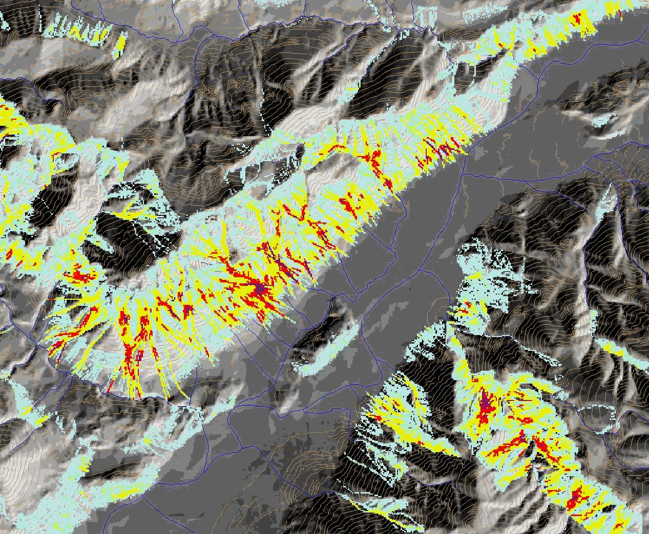
Raster outputs
computed by STONE. A) Rock fall counts. B) Rock fall velocity. C) Rock
fall flying height-
Vector outputs can take
different forms. For users interested in two-dimensional (planar)
representations of the rock-fall trajectories (i.e., in the production of maps
showing where rock-fall trajectories are located, and in the 2-D distribution of
rock-falls velocities and flying heights) STONE outputs two files, in ASCII
format, containing respectively:
-
the
ID (unique identifier) and the geographic (x and y) coordinates of the
points along the rock-fall trajectories; and
-
the
ID, elevation, velocity and flying height at each point along the
trajectories.
These files can be
imported into ArcInfo or ArcView , as well as other GIS and CAD systems. They
can be "joined" using the unique identifier (ID) and used to prepare
maps showing the spatial (planar) distribution of the rock-fall trajectories.
Points along the trajectories can be displayed with different symbols or colours
depending on velocity, flying height and travel mode.
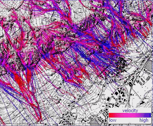
2-D vector trajectories
of rock-fall computed by STONE.
For users interested in
the three-dimensional display of rock-fall trajectories, STONE outputs an ASCII
file containing the x, y and z coordinates of all the points along the
trajectories, and the velocity and distance from the ground at each point. The
file can be read by three-dimensional CAD and GIS systems, provided that a
specific conversion program is available. A second ASCII file containing the 3
triplets of x, y, and z coordinates defining the local triangles used to compute
the rock-fall trajectories is also produced and can be used to help visualising
the rock-fall trajectories with respect to topography.
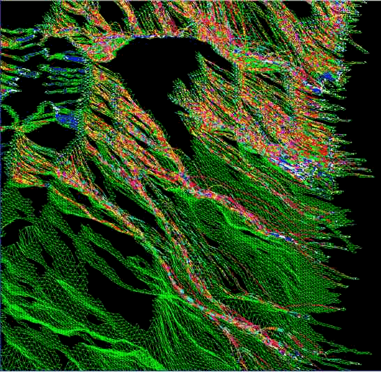
3-D vector trajectories
of rock-fall computed by STONE.
The size of the 2-D and
3-D vector files can become very large (easily exceeding 200 Mb for large
areas), depending on the user-controlled output resolution, the extent and
complexity of the study area, the number of source cells, the friction and
energy restitution coefficients, and the initial and minimum velocities set by
the user. Even if the dimension of the output files is limited only by computer
memory and disk space, in practice we prepared raster outputs for areas
exceeding 1400 km2 (i.e., 3.5 million cells with a ground resolution
of 20x20 meters), we prepared two-dimensional representation of rock-fall
trajectories for areas extending from few hectares to several tens of square
kilometres, and we displayed 3-D rock-fall trajectories for areas up to few
square kilometres.
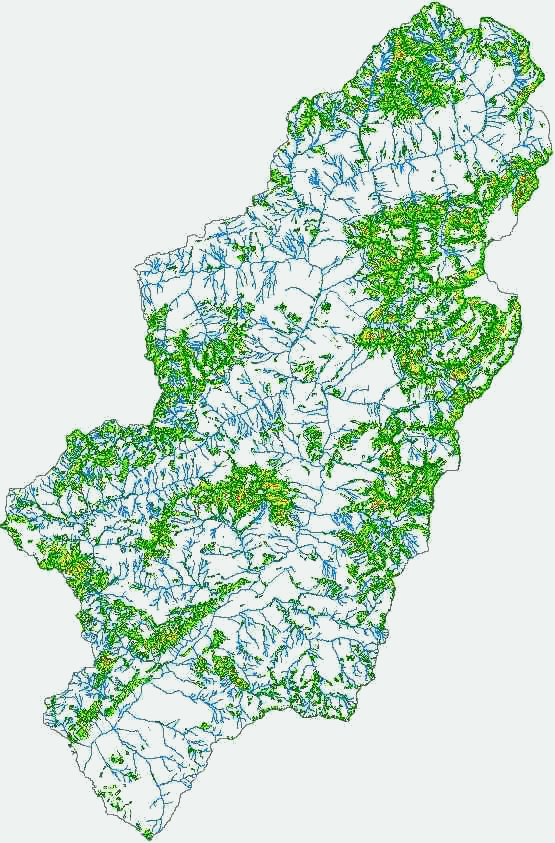
Rock
fall hazard map for the Camonica Valley, Lombardy. Northern Italy.
Parameters
such as the rock-fall starting velocity and direction, the dynamic friction
coefficient and the normal and tangential energy restitution coefficients
vary largely in nature and are difficult to define precisely, particularly over
large areas. STONE provides a way to cope with the natural
variability and local uncertainty associated with such information by adding to these
values a random component. The user can select a range of variation (in
percentage) around the given (default or central)
values. During the computation, where needed (i.e., at the beginning of a new
trajectory for the starting angle, at each impact point for the normal and
tangential energy restitution coefficients, and where the boulders rolls for the
dynamic friction coefficient), STONE draws randomly a value from the selected
range around the given (default) values. As an example, if a user selects the
ranges ± 3% and ± 2% for the normal and tangential energy restitution
coefficients respectively, and the values in the input grids for any given cell
are 50 and 65, respectively, STONE will select randomly a value for the normal
coefficient in the range 47-53 and a value for the tangential coefficient in the
range 63-67.
Values for the range of
variation are kept separated for the various input parameters. Thus, the normal
and/or tangential energy restitution coefficients can be varied separately
keeping the dynamic friction coefficient and the staring angle constant.
Similarly the starting angle can be selected
randomly keeping the parameters controlling the loss of energy constant. This
allows for flexible and complex simulations, and for
sensitivity analyses. If one or more of the selected ranges is set to
zero, STONE will use for that parameter the given (default) value.
The algorithm generating
pseudo-random numbers used by STONE needs an initiation seed. If the seed is
left unchanged, two successive runs of the program will provide exactly the same
results. This should be considered a positive feature because it allows to
replicate random simulations. To obtain completely different simulations the
value of the seed must be changed before each run. Thus, if the random component
is used to model rock-falls, separate runs of the program based on the same
input data and control parameters will provide the same results only if the seed
is the same, otherwise results will be different.
Adding the random
components to the simulation proves very useful to test the program outputs for
errors or inconsistencies due to local conditions. When
combined with the possibility of triggering a large number of boulders from each
starting cell (up to 1000), the use of the random components provides a way of
coping with the natural variability and the intrinsic uncertainty associated
with rock-falls. As a drawback the time required to complete a simulation
increases.
 
|


