


|
Rio
Lenzi Catchment

Basin
characteristics
The Rio Lenzi catchment is located within the Autonomous Province of Trento. Its main morphometric
characteristics are summarised in Table 1 and the location is shown in Fig. 1.
 |
|
| Catchment
area (km2) |
2.43 |
| Average
elevation (m a.s.l.) |
1880 |
| Minimum
elevation (m a.s.l.) |
1363 |
| Maximum
elevation (m a.s.l.) |
2409 |
| Mean
catchment gradient (%) |
53 |
| Length
of the main channel (km) |
2.29 |
| Main
channel mean gradient (%) |
26 |
|
|
Figure
1
|
|
Table
1
|
Settings
|
|
The geology of the catchment features an igneous upper
part, whilst the middle and the lower ones are characterised by quaternary morainic deposits
(see Fig. 2). The basin have a typical Alpine climate with annual precipitation
ranging from 930 to 1100 mm. Precipitation occurs mainly as snowfall from November to April. Runoff is usually dominated by
snowmelt in May and June whilst summer and early autumn floods
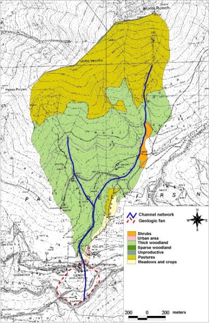
represent an important contribution to the flow regime. The vegetation cover mainly consists of forest stands made up by spruce
(Picea abies Karst.) and larch (Larix decidua Mill.); toward the timberline (at 1900 - 2100 m a.s.l.) the latter is associated with
Pinus cembra L. to form the last sparse woodlands before the ecological conditions impose shrubs (moorland) and
grasslands. A summary of the land use characteristics of the catchment is
reported in Tab. 2 and the map is reported in Fig. 3. |
|
Figure
2 |
|
|
The basins is prone to generate debris flows as it results from many
historical records.In the 1882 an extraordinary precipitation event occurred all around the Province of Trento, triggering a massive debris
flows along the Rio Lenzi stream. Several deep erosion (still active) were incised in the upper part, delivering huge amounts of sediment to
the main channel which built many lateral deposits downstream. The urbanised fan was flooded with severe damages. In 1917 and 1951
other smaller debris flow events affected the catchment fan. In the 1966 other extraordinary rainfalls produced a debris flow which
flooded on the lower part of the fan.
|
|
| Thick
woodland |
54% |
| Sparse
woodland |
0.3% |
| Shrubs |
0.9% |
| Grassland |
41.1% |
| Unproductive
(bare grounds, waterbodies, roads) |
2.9% |
| Urban
area |
0.3% |
|
| Table
2 |
Figure
3 |
DEM
implementation
|
|
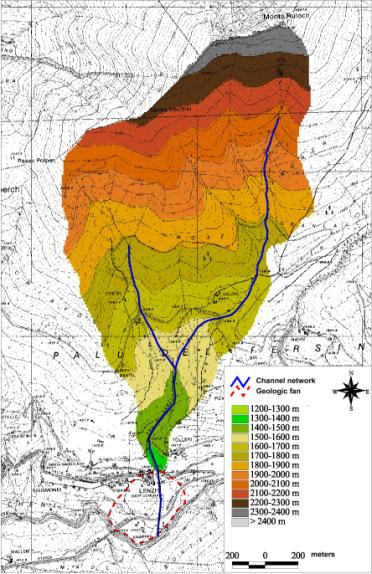
The GIS WODITEM (Watershed Oriented Digital Terrain Model) a
raster-type geographical information system especially devised for hydrological investigations in mountain basins, was used in order to
create the Digital Elevation Model (DEM) for the basin (Fig. 4), from which the slope and aspect raster maps were produced. A grid base of
10x10 m was used, apart from the Rio Lenzi fan where a 5x5 m grid was adopted. Pits were identified and removed in the raster elevation
map; a synthetic channel network was then extracted from the basin DEM. Digital Terrain Model (elevation, slope and aspect) and thematic maps
were created and edited using Arcview 3.1 software.
|
|
Figure
4 |
|
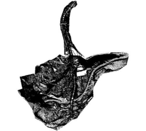
Fan Survey
|
In order to develop a physical based, user-friendly 1-D
(channel routing) and 2-D (propagation on the fan) models for the debris flow, a high-detailed elevation map is much
needed if the topography is assumed to be the determining factor upon the movement downstream of the flow, assumption which is taken to
simplify the numerous variables affecting the phenomenon. The existing topographic maps do not offer the proper accuracy
(1:1000 - 1:500 scale), therefore a high-precision topographic survey was needed for the fan area.
A classical survey methodology was adopted by using a total station system; the spatial density varied according to the local
morphology and to the proximity to the channel. In fact the survey methodology has to consider all the natural
(large boulders, past sediment heaps) and artificial (walls, roads, buildings) structures,
that might affect the debris flow trajectory. The fan DEM is shown in Figure 5.
|
|
|
Figure
5 |
|
|
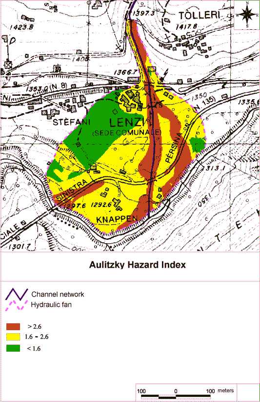
The Aulitzky methodology for debris flow hazard mapping was also
applied to the fan: the final map is shown in Fig. 6. The high precision of the elevation model obtained in this way will allow comparison with
quicker and cheaper survey techniques (GPS, photointerpretation, laser scanning
|
|
Figure
6 |
|


|